Outbound Holding time Adjustments
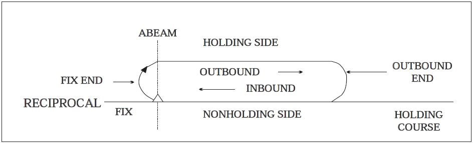
Holding patterns are designed by air traffic control to help delay aircraft for spacing, meter arrivals, or let them troubleshoot problems before they resume course. The goal is to fly in an oval racetrack pattern and stay within the confines of the space allocated by ATC to ensure safe flight.
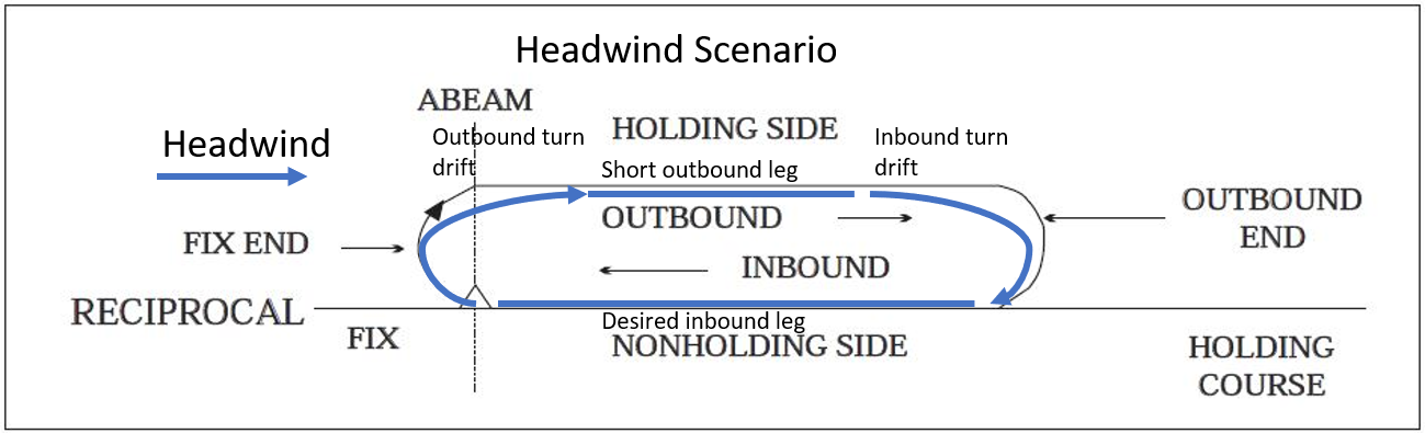
The turns need to be done at standard rate, so flying a nice semi-circular 180 in the airmass will yield a drift downwind over the ground. On the outbound turn, that will put us downwind of the abeam point. During the inbound turn, we’ll need to turn upwind of where we need to end up for our desired inbound leg. This means that our outbound leg will be shorter. In a tailwind scenario, the drift goes the other way, so we’d need a longer outbound leg. So, we know that we need drift corrections for the turns, and that these need to be added or removed from the outbound leg. Likewise, our ground speed in the outbound leg will be different, all of which will affect the timing.
The inbound leg is the easiest piece to solve for, and is also the one that we need to pin down to derive everything else. We know that distance = speed * time, so we can rearrange that to get what we need. Given fixed values, we know that our ground speed (GS) will be our TAS with a wind component offset (WC). By convention, let’s use negative values for headwinds and positive values for tailwinds. If, for example, we fly along at 100 KTAS with a 10-knot headwind, we’d write that as WC=-10, then add the values TAS+WC=GS, or 100+(-10)=90 kts GS. If we know how long our Ti needs to be, and we know our GS, we can compute the length of the inbound leg, Li. When working with Ti in minutes and speeds in knots (nautical miles per hour), we’ll also need to multiply or divide by 60 to get the correct units. Putting these components together into the gives us the following:
Li=[(TAS+WC)/60]*Ti
Going back to our example values above, with 100 KTAS and -10 WC, we get 90 kts GS, which when we divide by 60 gives us 1.5 nm/min. Multiplying by Ti=1 minute we get an Li of 1.5 nm. At and above 14,000 ft, ATC usually gives 1.5-minute holds, so let’s keep the Li as a variable even if it’s equal to 1 for most low-altitude work.
Next up, let’s go back to our sketch and find the next piece to solve, namely the turns. Because the turns are flown at a standard rate, they form a perfect semi-circle through the airmass (assuming we fly precisely…). Thus, we just need to compute the total wind drift (Dw) in the turns. We know that we’ll do two turns, and that each will take one minute (barring crosswind corrections), so we end up with the following:
Dw=2*(WC/60)
When we simplify that, we get:
Dw=WC/30
Back to our sample problem, our 10-knot (.1667 nm/min) headwind (WC=-10) for two minutes gives us -.333 nm of total drift.
Next, we need to solve for the outbound leg distance, or Lo. Going back to the sketch, we know that it needs to be shorter than Li in a headwind scenario (WC<0), and longer in a tailwind scenario (WC>0). If Dw is negative in a headwind, as per our convention, then we simply add it to Li to get the following:
Lo=Li+Dw=[(TAS+WC)/60]*Ti+WC/30
In the example we’re using, that means Lo=1.5 nm -.333 nm = 1.166 nm
Lastly, we need to combine our outbound GS with Lo to determine To. This means rearranging the equation to be time = distance / speed. This time round, we need to subtract WC from TAS because we’re going the other way. Thus, we end up with the following:
To=Lo/[(TAS-WC)/60]
In our case, that means:
To=1.166/[(100-(-10)/60] = 1.16/(110/60) = 1.16/1.833=.6363 minutes, or 38 seconds
Putting that whole equation back together in terms of the original inputs yields this incredibly ugly equation:
To={[(TAS+WC)/60]*Ti+WC/30}/[(TAS-WC)/60]
We can simplify a bit to get this:
To=[(TAS+WC)*Ti+2WC]/(TAS-WC)
Cool, now we’ve accomplished goal #1, but I wager that few pilots will consistently be able to compute that accurately while flying the plane in IMC and dealing with all the other workload like briefing the next approach, setting up the box, etc. When confronted with these sorts of situations, pilots come up with approximations that are close enough to fly the plane well enough without spending too much time doing math. For the sake of this, let’s fix a few variables, namely TAS=100 knots and Ti=1 minute, or 60 seconds. Let’s use a range of winds from -35 knots to +35 and see what we get:
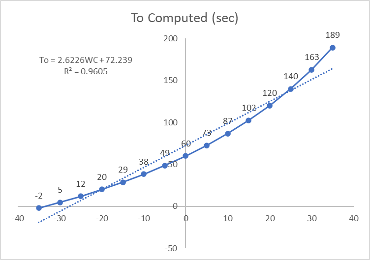
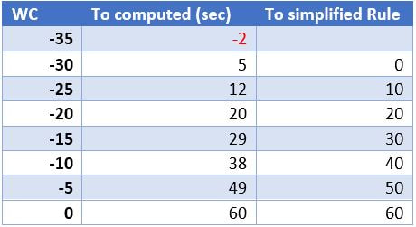
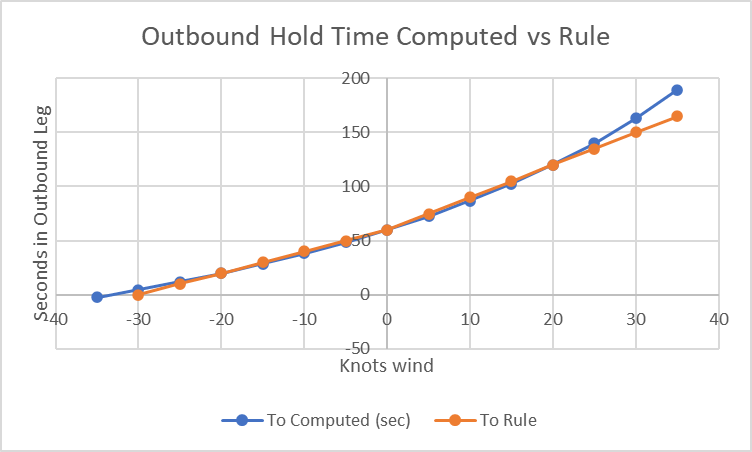
Our output is a curving line with wind on the horizontal and time on the vertical. On the left, we see that at -35 knots, the outbound leg time is negative, and it’s only 5 seconds at -30 knots. Basically, this means that with a headwind around 33 knots, the drift distance alone will take us beyond Li, so we should skip the outbound leg entirely and just fly both turns back-to-back. The regression output To=2.62WC+72 is not exactly easy to remember either, so let’s think of a better approximation that we can easily recall. At WC=-30, the To can be approximated to 0, and we know it needs to be 60 seconds at WC=0, so drawing a straight line between those gives us, in seconds, To=60+2WC. Comparing the rule to the computed values shows us that the error is pretty small:
In the tailwind scenario, the curve in the chart above steepens and the 2x rule falls apart pretty quickly. If we instead put in 3x for To=60+3WC, we get this:
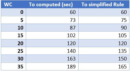
Overall, the 2x headwind and 3x tailwind is good enough until you get to a 30-knot tailwind:
Putting this all together, here are the simplified rules:
At 100 KTAS: for every knot of headwind, subtract 2 seconds outbound.
At 100 KTAS: for every knot of tailwind, add 3 seconds outbound.
This works pretty well for a TAS around 100 knots. For grins, I tried to create a rule at 200 KTAS, and found that 1 second per knot headwind and 1.5 second per knot tailwind get you pretty close:
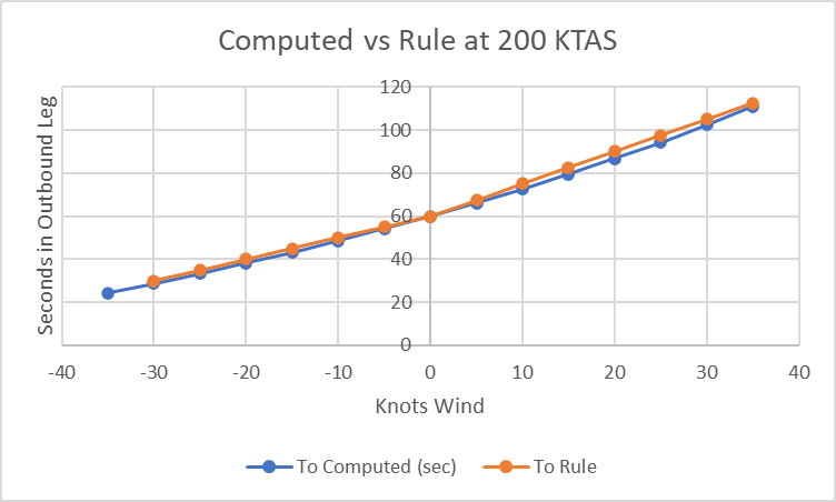
Thinking about the relationships between the TAS=100 and the TAS=200 case, a generic rule for a range of holding TAS can be made as follows:
For every knot of headwind, subtract 200/TAS seconds outbound.
For every knot of tailwind, add 300/TAS seconds outbound.
Example: at 150 KTAS in a 10-knot tailwind, you’d add (300/150) * 10 = 20 seconds to your outbound time.
In this example, the computed outbound leg value is 77 seconds, and the rule gives you 80 seconds. Close enough….
Keep in mind that these values are for 1-minute holds. Hopefully this helps you all have more precise inbound leg times, or provides a good brain teaser for your students. Happy landings!